Okay now let's start with our lesson today is to get a table.
First run your Microsoft Office Excel by clicking Start - All programs - Microsoft Office - Microsoft Office Excel 2003 (for those who use another version of Microsoft Office such as Microsoft Office 97, Microsoft Office 2000, Office XP Office Microsoft, not a problem). note the following images :

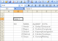
After the worksheets are in Microsoft Office Excel, make a table like the following picture:

How:
Place the pointer on the cell B3 and then type in Table 1 and Enter
Next place the pointer on cell B5 and typing NO then Enter
The next step place the pointer in cell B6 and type the numbers 1 (do this step until the cell B10 to make Number Sort).
After a number Sort, now we make a column name, the way same way over the place the pointer on the right C5 No. column on the right.
Do this until the complete address and the City so the result will look like the picture above.
When finished making the table above, now we must set the column width to fit the width of the data (text / number) that the inputs on each of each cell.
The trick is:
Because here we are just changing the column width for the placement of the pointer must be akolom pad that will be changed in size, while the line-free. Suppose you want to change the width of column B aka pointer must be in column B and the line could be in line 1, 2, 3 and so on until the very last row.
Change column Table 1 above that you created with the following sizes:
Column B: 4.43
Column C: 12
Column D: 22
Column E: 12
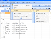
How: to change the width of column B, place the pointer in cell B1 or B2 or B3, and so on and then click the Format menu - Column - Width, and then enter or type the number for the column width of 4.43 and press Enter. View images :

After changing the width of column B, then change the width of column C = 12, D = E = 22 and 12 do follow the way to change the width column B above.
After all, save the file with the file name TABEL1.XLS, by clicking File Menu - Save As and then typing the name TABEL1 file and click save.